Chapter – 1
Physics and Measurement
Syllabus
Physics, technology and society, S I Units, fundamental and derived units, least count, accuracy and precision of measuring instruments, Errors in measurement, Dimensions of Physics quantities, dimensional analysis and its applications.
Physics, Technology and Society
Physics, Technology and society depend upon each other for their existence. There are instances where physics gives rise to technology and there also have been instances where technology gave rise to physics. Physics tells the society about natural phenomena, energy laws and basic tech knowledge whereas technology helps the society practically by making their life easier. This article deals with how the three of them are interrelated and interdependent.
Examples to relate physics, technology and society :
- How technology gave rise to physics :Principles of thermodynamics and magnetism originated keeping in mind the already existing technology related to them. These principles were required to have an in-depth, calculative knowledge of the topic and to make some advancements in the previously existing technology by deeply studying them and experimenting with them. This was possible only because of the already prevailing technology. People earlier had known about the magnetic effect but due to lack of knowledge of the reason behind that effect, they were unable to understand and explain it. Hence, people progressed in this field only after physics and technology were combined and they could have a complete knowledge about it.
- How physics gave rise to technology:Now, we all know that wireless communication technology was formed by using and following the principles of electricity and magnetism. Moreover, only by studying the laws of physics related to energy, we are now able to form technology that can conserve wind energy, solar energy, hydra energy etc,. This has helped us to conserve our fossil fuels. We can convert these stored energies into electrical energy. This was all possible because of absolute knowledge of physics that could contribute to the formation of this technology. The human course of civilization was hugely impacted after the invention of the steam engine in the 18th century.
Physicists and their contributions
| Name | Contributions/Discoveries | Country/Origin |
|---|---|---|
| Archimedes | Principle of buoyancy; Principle of the lever | Greece |
| Galileo Galilei | Law of inertia | Italy |
| Christiaan Huygens | Wave theory of light | Holland |
| Isaac Newton | Universal law of gravitation; Laws of motion; Reflecting telescope | U.K. |
| Michael Faraday | Laws of electromagnetic induction | U.K. |
| James Clerk Maxwell | Electromagnetic theory; Light-an electromagnetic wave | U.K. |
| Heinrich Rudolf Hertz | Generation of electromagnetic waves | Germany |
| J.C. Bose | Ultra short radio waves | India |
| W.K. Roentgen | X-rays | Germany |
| J.J. Thomson | Electron | U.K. |
| Marie Sklodowska Curie | Discovery of radium and polonium; Studies on natural radioactivity | Poland |
| Albert Einstein | Explanation of photoelectric effect; Theory of relativity | Germany |
| Victor Francis Hess | Cosmic radiation | Austria |
| R.A. Millikan | Measurement of electronic charge | U.S.A. |
| Ernest Rutherford | Nuclear model of atom | New Zealand |
| Niels Bohr | Quantum model of hydrogen atom | Denmark |
| C.V. Raman | Inelastic scattering of light by molecules | India |
| Louis Victor de Broglie | Wave nature of matter | France |
| M.N. Saha | Thermal ionisation | India |
| S.N. Bose | Quantum statistics | India |
| Wolfgang Pauli | Exclusion principle | Austria |
| Enrico Fermi | Controlled nuclear fission | Italy |
| Werner Heisenberg | Quantum mechanics; Uncertainty principle | Germany |
| Paul Dirac | Relativistic theory of electron; Quantum statistics | U.K. |
| Edwin Hubble | Expanding universe | U.S.A. |
| Ernest Orlando Lawrence | Cyclotron | U.S.A. |
| James Chadwick | Neutron | U.K. |
| Hideki Yukawa | Theory of nuclear forces | Japan |
| Homi Jehangir Bhabha | Cascade process of cosmic radiation | India |
| Lev Davidovich Landau | Theory of condensed matter; Liquid helium | Russia |
| S. Chandrasekhar | Chandrasekhar limit, structure and evolution of stars | India |
| John Bardeen | Transistors; Theory of super conductivity | U.S.A. |
| C.H. Townes | Maser; Laser | U.S.A. |
| Abdus Salam | Unification of weak and electromagnetic interactions | Pakistan |
| Sudarshan | V A theory of weak interaction | India |
Physical Quantities
The quantities which can be measured by an instrument and by means of which we can describe the laws of physics are called physical quantities.
For examples,
Newton’s Law of Motion: F = m x a , This law has been described by three physical quantities namely, Force (F), Mass (m) and Acceleration (a).
Ohm’s Law: V = I x R , This law has also been described by three different physical quantities, namely, Potential difference (V), Electric current (I) and Electric resistance (R).
Similarly, all physical relations derived in physics can be derived by different physical quantities. Some examples of physical quantities: mass, length, time, velocity, acceleration, force, Gravitational field, Refractive Index, electric charge, electric current etc.
Types of Physical Quantities:
There are three types of physical quantities. They are –
(i) Fundamental or Basic Quantities,
(ii) Derived Quantities and
(iii) Supplementary Quantities
Fundamental Quantities: The quantities that do not depend upon any other quantities are called fundamental or absolute or basic
quantities.
There are seven fundamental quantities:
(i) Length, (ii) Mass, (iii) Time, (iv) Temperature, (v) Electric current, (vi) Luminous of Intensity and (vii) Amount of Substance
Derived Quantities: The quantities which are derived from fundamental quantities are known as derived quantities. Eg., area, volume, density, force, work, electric current etc.
Here, Area = [length]2 , derived from length,
Force = mass x length x (time)-2, derived from mass, length and time etc.
Supplementary Quantities: Besides seven fundamental quantities, two supplementary quantities are also defined. They are:
(i) Plane angle (ii) Solid angle
Physical Units
Measurement:
The measurement of a physical quantity is the process of comparing this quantity with a standard which has the same nature as the quantity to be measured is chosen. It is called the unit.
Expression of a physical quantity:
Any physical quantity (Q) can be expressed as a number (n) times the unit (u).
i.e., Q = n x u
If the unit (u) is changed, then (n) also changes such the product or magnitude of Q always remains constant. Therefore,
Q = n1u1 = n2u2
Eg., mass of a body, m = 4 kg = 1000 g.
Smaller the units, larger the numerical value.
Physical Unit:
The chosen standard of same kind taken as reference for the measurement of physical quantity is called as the unit of that quantity.
Requirement of a physical unit:
It should be
(a) of suitable size
(b) accurately defined
(c) easily accessible
(d) easily reproductible
(d) not change with time, temperature, pressure etc.
(e) internationally acceptable
(f) easily accessible.
Types of Physical Units:
(i) Fundamental units:
The physical units which can neither be derived from one another, nor they can be further resolved into more simpler units are called fundamental units.
In other words, the units of fundamental quantities are called fundamental units. For examples:
units of length: metre, centimetre, foot etc.
units of mass: kilogram, gram, pound etc.
units of time: second, minutes, hours, years etc.
(ii) Derived units:
All the other physical units which can be expressed in terms of the fundamental units are called derived units. In other words, the units of derived quantities are called derived units.
Example:
Force = mass x acceleration = mass x displacement/time2
Unit of force = kg x m/s2 = kgms-2
System of Units:
A complete set of units which is used to measure all kinds of fundamental and derived quantities is called a system of units. There are four commonly used system are units. They are
(i) CGS system: The system of units in which length, mass and time are measured in centimetre, gram and second respectively is called CGS system of units. It is a French
system of units.
(ii) FPS system : The system of units in which length, mass and time are measured in foot, pound and second respectively is called FPS system of units. It is a British system of units.
(iii) MKS system: The system of units in which length, mass and time are measured in metre, kilogram and second respectively is called MKS system of units. This is also mass and time are measured in metre, kilogram and second respectively is called MKS system of units. This is also a French system of units.
SI units
It is an abbreviation of ‘Le systems International d ‘unites’ which is French equivalent of international system of units. It is extended form of MKS system of units in course of acquiring all fundamental units instead of three as in MKS system of units. This was adopted by 11th General conference of Weights and Measures in 1960.
Fundamental units
| Fundamental Quantities | Symbol | Fundamental Units | Symbol |
|---|---|---|---|
| Length | l | meter | m |
| Mass | m | kilogram | kg |
| Time | t | second | s |
| Temperature | T | kelvin | K |
| Electric Current | I | ampere | A |
| Luminous Intensity | I | candela | cd |
| Amount of Substance | __ | mole | mol |
| Supplementary Quantities | Symbol | Fundamental Quantities | Symbol |
| Plane angle | θ | radian | rad |
| Solid angle | Ω | steradian | sr |
Definitions of Fundamental SI units:
1. Metre (m): It is defined by taking the fixed numerical value of the speed of light in vacuum c to be 299792458 when expressed in the unit m s–1, where the second is defined in terms of the caesium frequency Δvcs.
2. Kilogram (kg): It is defined by taking the fixed numerical value of the Planck constant h to be 6.62607015×10⁻³⁴ when expressed in the unit J s, which is equal to kgm2 s–1, where the metre and the second are defined in terms of c and Δvcs.
(3) Second (s): One second is the duration of 9,192,631,770 periods of the radiation corresponding to the transition between two hyperfine levels of the ground state of the caesium-133 atom.
(4) Kelvin (K): One kelvin is the fraction 1/273.16 of the thermodynamic temperature of the triple point of water. The triple point of water is the temperature at which ice, water and water vapour co-exist.
(5) Ampere (A): One ampere is that constant current which, if maintained in two straight parallel conductors of infinite length, of negligible cross-section and placed 1 metre apart in vacuum, would produce between these conductors a force equal to 2 x 10⁻⁷ newton per metre of length.
(6) Candela (cd) : One candela is the luminous intensity, in a given direction, of a source that emits monochromatic radiation of frequency 540 x 1012 hertz and that has a radiant intensity of 1/683 watt per steradian in that direction.
(7) Mole (mol): One mole is that amount of a substance which contains as many elementary entities(atoms, mol ecules or ions) as there are atoms in 0.012 kg of carbon12 isotope.
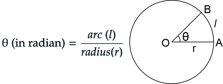
(8) Radian (rad): It is defined as the plane angle subtended at the centre of a circle by an arc equal in length to the radius of the circle.
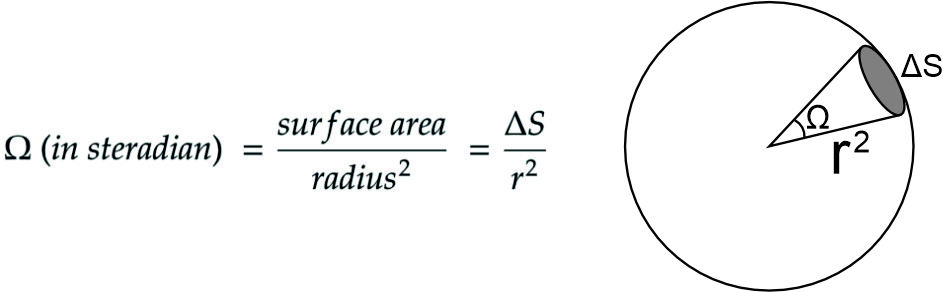
(9) Steradian (sr): It is defined as the solid angle subtended at the centre of a circle by an arc equal in length to the radius of the circle.
Guideline for writing SI units in symbol
(i) Small letters are used for symbols of units.
(ii) Symbols are not end with a full stop.
(iii) Capital initial letter is used only if the unit is named after a scientist.
(iv)Symbols do not take plural form.
(v)The full name of a unit always begins with a small letter even if it has been named ager a scientist. For example, SI unit of Force is N or newton.
Expression of large magnitude of physical quantity in power of 10
For example, mass of a box is 2000 g.
m = 2000 g = 2 x 10³g = 2 kg
Here, ‘k’ is the prefix used for 1000 (103).
Similarly, the magnitude of physical quantities is over a wide range. So in order to express the very large magnitude as well as very small magnitude more compactly, “CGPM” recommended some standard prefixes for certain power of 10.
| SI Prefix | Symbol | Power | SI Prefix | Symbol | Power |
|---|---|---|---|---|---|
| yotta | Y | 1024 | yocto | y | 10-24 |
| zetta | Z | 1021 | zepto | z | 10-21 |
| exa | E | 1018 | atto | a | 10-18 |
| peta | P | 1015 | femto | f | 10-15 |
| tera | T | 1012 | pico | p | 10-12 |
| giga | G | 109 | nano | n | 10-9 |
| mega | M | 106 | micro | μ | 10-6 |
| kilo | k | 103 | milli | m | 10-3 |
| hecto | h | 102 | centi | c | 10-2 |
| deca | da | 101 | deci | d | 10-1 |
Derived Units
| Derived quantities | Formula | Derived SI Units |
|---|---|---|
| Speed | $$\frac{distance}{time}$$ | ms-1 |
| Velocity | $$\frac{displacement}{time}$$ | ms-1 |
| Acceleration | $$\frac{velocity}{time}$$ | ms-2 |
| Linear momentum | mass x velocity | kgms-1 |
| Force | mass x acceleration | kgms-2 or newton (N) |
| Impulse | Force x time | kgms-1 or Ns |
| Pressure | $$\frac{force}{area}$$ | kgm-1s-2 or Nm-2 or pascal (Pa) |
| Work or Energy | Force x displacement or Capacity of doing work | kgm2s-2 or Nm or joule (J) |
| Power | $$\frac{work}{time}$$ | kgm2s-3 or watt (W) |
| Torque | force x perpendicular distance | kgm2s-2 or Nm |
| Gravitational constant (G) | $$\frac{force{\times}distance^2}{mass^2}$$ | kg-1m3s-2 or Nm2kg-2 |
| Stress | $$\frac{Restoring\ force}{area}$$ | Nm-2 |
| Strain | $$\frac{change\ in\ dimension}{original\ dimension}\mathrm{\ }$$ | unitless |
| Coefficient of Elasticity | $$\frac{stress}{strain}$$ | Nm-2 |
| Surface tension | $$\frac{force}{length}$$ | Nm-1 |
| Surface energy | $$\frac{Energy\ stored}{area}$$ | Jm-2 |
| Coefficient of Viscosity | $$\frac{force}{area{\times}velocity\ gradient}\mathrm{\ }$$ | kgm-1s-1 or Nm-2s or Poiseuille |
| Angular velocity | $$\frac{angular\ displacement}{time}$$ | rad s-1 |
| Angular acceleration | $$\frac{angular\ velocity}{time}$$ | rad s-2 |
| Angular momentum | Linear momentum x perpendicular distance | Kgm2s-1 |
| Moment of inertia | mass x distance2 | kgm-2 |
| Frequency | $$\frac{1}{time\ period}$$ | s-1 or hertz (Hz) |
| Planck’s constant | $$\frac{energy}{frequency}$$ | kgm2s-1 or J s |
| Specific heat | $$\frac{heat}{mass{\times}change\ in\ temperature}$$ | J Kg-1K-1 |
| Latent heat | $$\frac{heat}{mass}$$ | J kg-1 |
| Thermal conductivity | $$\frac{rate\ of\ flow}{area{\times} temperature gradient}$$ | Js-1m-1K-1 |
| Entropy | $$\frac{heat\ change}{temperature\ change}$$ | JK-1 |
| Universal gas constant | $$\frac{pressure{\times}volume}{no\ of\ moles{\times} temperature}$$ | J mol-1 K-1 |
| Boltzmann constant | $$\frac{Universal\ gas\ constant}{Avogadro’s\ number}$$ | J K-1 |
| Stefan’s constant | $$\frac{Energy}{time{\times} area{\times} temperature^4}$$ | J s-1 m-2 K-4 |
Accuracy and Precision
Accuracy: The accuracy is defined as the closeness of the measured value to the true value of a physical quantity.
(i) It indicates the relative freedom from errors. As we reduce the errors, the measurement becomes more accurate.
(ii) The problem of accuracy is arises due to errors like human errors, method error, instrument error etc.
(a) The human error can be avoided by repeating the measurement and recording them carefully.
(b) The method error can be minimized by standardizing the method of taking measurement.
(c) The instrumental error can be minimized by using high quality instruments.
For example, the true value of ‘g’ is 9.8 m/s2. Let its measured value be 9.75 m/s2 and 9.79 m/s2. Then the more accurate value is 9.79 m/s2 because it is more close to the true value 9.8 m/s2 .
.
Precision: It is defined as the degree of exactness of a measurement.
(i) It indicates as to what smallest limit a physical quantity can be measured.
(ii) In fact, it is a measure of the limitation of a measuring instrument.
For example, the least value of any measurement made by a vernier callipers is 0.01 cm and for another calliper is 0.001cm. Then the second calliper has more precision.
(iii) The lack of precision is due to limitation of the instrument. In fact, precision of a measurement is determined by the least count of measuring instrument. Smaller is the least count, greater is the precision.
(iv) If we repeat a particular measurement of a quantity a number of times, then the precision refers to the closeness between the different observed values of the same quantity.
(v) High precision does not mean high accuracy.
For example, Suppose three students are asked to find the length of a rod whose length is known to be 2.250 cm. The observations data are given in the table.
| Student | Measurement I (in cm) | Measurement II (in cm) | Measurement III (in cm) | Average (in cm) |
|---|---|---|---|---|
| A | 2.25 | 2.27 | 2.26 | 2.26 |
| B | 2.252 | 2.250 | 2.251 | 2.251 |
| C | 2.250 | 2.250 | 2.251 | 2.250 |
Conclusion:
(i) Student A: Neither precise nor accurate.
(ii) Student B: More precise but not accurate.
(iii)Student C: Both precise as well as accurate.
Least count of a measuring instrument
Least Count (LC): Least count of a measuring instrument is the smallest value that can be accurately measured using this instrument.
For example,
(i) Least count of vernier callipers
$$L.C.\ =\ \frac{Value\ of\ 1\ main\ scale\ division}{Total\ number\ of\ vernier\ scale\ division}$$
(ii) Least count of screw sauge
$$L.C.\ =\ \frac{Value\ of\ 1\ pitch\ scale\ reading}{Total\ number\ of\ circular\ scale\ division}$$
Note: For detail of the instruments, read JEE Advanced General Physics. Click here
Significant figures
The significant figures are normally those digits in a measured quantity which are known reliably or about which we have confidence in our measurement plus one additional digit that is uncertain.
(a) The larger the number of significant figures in a measurement, the higher is the accuracy of the measurement.
(b) It indicates the degree of precision of measurement.
(c) The degree of precision is determined by the least count of the measuring instrument.
Suppose a length measured by
(i) a metre scale (of least count = 0.1 cm) is 1.5 cm, then it has two significant figures, namely 1 and 5 in which 1 is reliably known and 5 is uncertain.
(ii) a Vernier callipers (of least count = 0.01 cm) the same length is 1.53 cm and it then has three significant figures, namely 1, 5 and 3, out of which 1 and 5 are certain and 3 is uncertain.
(iii) a screw gauge ( of least count = 0.001 cm) the same length may be 1.536 cm which has four significant figures, out of which right most digit i.e., 6 is uncertain.
Hence, smaller the value of least count, more is the significant figure.
Rules to Determine the Number of Significant Figures:
(i) All the non-zero digits are significant. Example, 14,245 contains five significant figures.
(ii) All the zeros between two non-zero digits are significant no matter where the decimal point is. For example, 104.009 contains six significant figures.
(iii) If the number is less than 1, the zeros on the right of decimal point but to the left of 1st non-zero digit are not significant. For example, 0.0012407 has five significant figure. Underlined zeros are not significant figures.
(iv) All the zeros to the right of the last non-zero digit (trailing zero) in a number without a decimal point are not significant. For example, 453 m = 45300 cm = 453000 mm has three significant figures. The trailing zeros are not significant but if these are obtained from a measurement, they are significant.
(v) The trailing zeros in a number with a decimal point are significant. For example, 3.500 or 0.003600 has four significant figures.
Notes:
(a) We cannot increase the accuracy of a measurement by changing the unit.
For example, if the mass of a body is 36.4 kg. It means that measuring instrument has a least count of 0.1 kg. In this measurement, three figures 3, 6 and 4 are significant.
If we change 36.4 kg to 394000 g or 394000000mg, we cannot change the accuracy of measurement.
Hence, 394000 g or 394000000 mg still have three significant figures; the zeros only serve to indicate only the magnitude of measurement.
(b) If we don’t know least count of the measuring instrument, then we cannot be sure that last digits (zeros) are significant or not.
(c) There can be some confusion regarding the trailing zero(s). Suppose a length is reported in a scale to be 2.800 m. Now suppose we change units, then 2.800 m = 280.0 cm = 2800 mm = 0.002800 km. Since the last number has trailing zeros in a number with no decimal (2800 cm), we would conclude that the number has two significant figures, while in fact, it has four significant figures and a mere change of units cannot change the number of significant figures.
To remove such ambiguities in determining the number of significant figures, the best way is to report every measurement measurement in scientific notation i.e., in the power of 10.
(d) Scientific Notation: In scientific notation, every number is expressed as N x 10n ,where ‘N’ is a number between 1 and 10 i.e., decimal point is always placed after 1st non-zero digit. and ‘n’ is any positive or negative exponent (or power) of 10.
For example,
2.800 m = 2.800 x 102 cm = 2.800 x 103 mm = 2.800 x 10⁻³ km
The power of 10 is irrelevant to the determination of significant figures. However, all zeros appearing in the base number in the scientific notation are significant. Each number in this case has four significant figures.
Rules for Arithmetic Operations with Significant Figures:
(i) In multiplication or division, the final result should retain as many significant figures as are there in the original number with the least significant figures.
For example, If mass and volume of a wooden ball are 4.237g (four s.f.) and 2.51 cm3 (three s.f.) respectively then the density of the ball should be
Density =\(\frac{4.237\ g}{2.51\ cm^{3}}\) = 1.69 g cm-3 (three s.f.)
(ii) In addition or subtraction, the final result should retain as many decimal places as are there in the number with the least decimal places. For example,
Addition:
436.32 g (five s.f.) + 227.2 g (four s.f.) + 0.301 g (three s.f.) = 663.821 g. But the least precise measurement (227.2 g) is correct to only one decimal point. Therefore, the final result should be rounded off to 663.8 g.
Subtraction:
0.307 m – 0.304 m = 0.003 m = 3.00 x 10⁻³ m (three S.F)
Round Off the Uncertain Digit (Least Significant Digit)
The least significant digit is rounded according to the rules:
- If the digit next to the least significant (Uncertain) digit is more than 5, the digit to be rounded is increased by 1.
- If the digit next to the rounded one is less than 5, the digit to be rounded is left unchanged.
- If the digit next to the rounded one is 5, then the digit to be rounded is increased by 1 if it is odd and left unchanged if it is even.
The insignificant digits are dropped from the result if they appear after the decimal point. Zero replaces them if they appear to the left of the decimal point.
Error in Measurement
Error: The difference between the true value and observed value of any physical quantity is called the error of measurement.
Error = True value – observed value
(i) Whenever we measure a physical quantity, the value observed is never exactly equal to the true value. Every measurement has an error.
(ii) An error gives an indication of the limits within which the true value may lie.
Types of Errors:
(1) Constant errors: The errors which affect the observation by the same amount are called constant errors.
Cause: Due to faulty calibration of the scale of the measuring instrument.
Correction: It can be minimised by measuring the same quantity by a number of different methods, apparatus or technique.
(2) Systematic errors: The errors which tend to occur of one sign, either positive or negative, are called systematic errors. In other words, the errors whose causes are known to us are called systematic errors.
Cause: It occurs due to some known cause which follow some specified rule. It may occur due to zero error of an instrument, imperfection in experimental techniques, change in weather condition like temperature, pressure etc.
Correction: If we know their cause, we can eliminate it.
Types of Systematic errors based on their cause:
(a) Instrumental error: These errors occur due to the inbuilt defect of the measuring instrument.
For example, zero error in a vernier callipers i.e., zero of the vernier scale may not coincide with the zero of the main scale.
Correction: It can be minimized by using a more accurate instrument.
(b) Imperfections in experimental technique: These errors occur due to the limitations of the experimental arrangement.
For example, error due to radiation loss in calorimetric experiments.
Correction: It can not be eliminated but necessary corrections can be applied for them.
(c) Personal errors: These occurs due to individual’s bias, lack of proper setting of apparatus or individual’s carelessness in taking observations without observing proper precautions, etc.
For example, when an observer holds his head towards right, while reading a scale, he does some errors due to parallax.
Correction: It can be minimized if measurements are repeated by different persons on removing the personal bias as far as possible.
(d) Errors due to external causes: These occurs due to change in external conditions like pressure, temperature, winds etc.
For example, the expansion of a scale due to the increase in temperature.
Correction: It can be minimized by controlling the external conditions during the experiments.
(3) Random errors: The errors which occur irregularly and at random, in magnitude and sign are called random errors. In other words, the errors whose causes are not known to us are called random errors.
Cause: It occurs by chance and arise due to uncontrollable conditions affecting the observer, measuring device and quantity to be measured. These errors are neither systematic nor constant but are equally likely to be positive or negative.
Correction: It can not be corrected because its causes are not known to us. These errors can be minimised by taking more and more readings and computing the arithmetic mean. This arithmetic mean of large number of observation can be taken as the true value of the measured quantity.
(4) Gross errors: The errors which occur due to either carelessness of person or due to improper adjustment of the instrument are called gross errors.
For example, recording the observations wrongly, using wrong values of the observations in calculations, ignoring sources of errors, etc.
Correction: No correction can be applied but can be minimised only when the observer is sincere.
(5) Least count errors: The errors which occur due to the limitations imposed by the least count of the measuring instrument are called least count errors.
(a) It is an uncertainty associated with the resolution of the measuring instrument.
(b) The smallest division on the measuring instrument is called its least count.
(c) The maximum possible error is equal to the least count.
For example, the least count of
(a) meter scale is 0.1 cm.
(b) vernier scale is 0.01 cm and
(c) screw gauge is 0.001 cm.
The readings are good up to these values.
Correction: These errors can only be corrected by choosing the right instrument to take measurement.
Eliminations of Random errors:
The random errors can be minimized by repeating the observation a large number of times and taking the arithmetic mean of all the observations. The mean value can be taken as the true value of the observed quantity.
If a1, a2, a3, ………………. an, are the observed value of a quantity then true value amean can be given as
$$a_{mean} =\frac{a_{1} +a_{2} +a_{3} +……….+a_{n}}{n}\mathrm{\ }$$
(i) Absolute errors: The difference between the true value and the measured value of a quantity is called an absolute error. Usually the mean value amean or am is taken as the true value. So, if
$$a_{m} =\frac{a_{1} +a_{2} +a_{3} +……….+a_{n}}{n}\mathrm{\ }$$
Then, absolute errors in the measured values of the quantity are,
Δa1 = am – a1
Δa2 = am – a2
Δa3 = am – a3
…………………………
…………………………
Δan = am – an
Absolute error may be positive or negative.
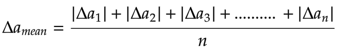
(ii) Mean absolute error: It is the arithmetic mean of the magnitudes of absolute errors. Thus,
The final result of measurement can be written as
a = am ± Δamean
This implies that value of ‘a‘ is likely to lie between am + Δamean and am – Δamean.
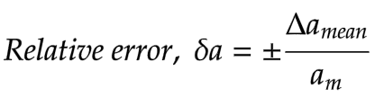
(iii) Relative or Fractional error: The ratio of mean absolute error to the mean value of the quantity measured is called relative or fractional error. Thus
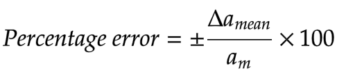
(iv) Percentage error: The relative error expressed in per centage is called as the percentage error i.e.,
Combination of Errors:
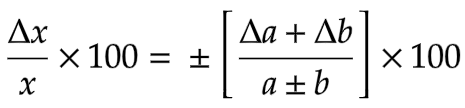
(1) Errors in sum or difference: Let x = a ± b. If Δa be the absolute error in the measurement of a, Δb the absolute error in the measurement of b and Δx is the absolute error in the measurement of x, then maximum absolute error in x is
Δx = Δa ± Δb
Note:
(i) The maximum value of Δa and Δb can be least count of the instrument used. For example, if a = 2.20 cm, Δa will be 0.01 cm.
(ii) Percentage error in ‘x’ is given as
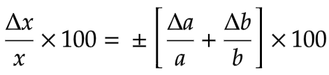
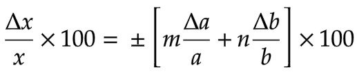
(2) Error in product or quotient: Let x = ab or a/b, then maximum relative error of x is
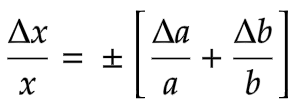
Maximum percentage error in x is
(3) Error in quantity raised to some power: Let x = am x bn or am/bn then maximum relative error in x is

Maximum percentage error in x is
Different methods of calculating errors:
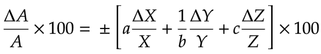
(1) Let $$A=\frac{X^{a}\sqrt[b]{Y}}{Z^{c}}$$
Maximum relative error in A is
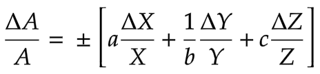
Maximum percentage error in A is
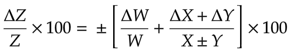
(2) Let $$Z=\frac{W}{X\pm Y}$$
Then maximum relative error in Z is
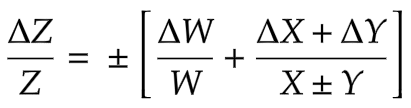
Maximum percentage error in Z is
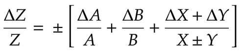
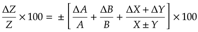
(3) Let $$Z=\frac{AB}{X\pm Y}$$
Then maximum relative error in Z is
Maximum percentage error in Z is
(4) Let
z = sin x
Then maximum relative error in z is
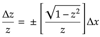
Maximum percentage error in z is
Dimension of a physical quantity
Dimensions of a physical quantity are the powers to which the fundamental quantities must be raised to express that quantity.
For example,
$${density = \frac{mass}{volume}=\frac{mass}{(length)^3}}$$
or, $${density = (mass)(length)^{-3}}$$
Thus, the dimensions of density are 1 in mass and -3 in length. The dimensions of all other fundamental quantities are zero.
Dimensions of Fundamental quantities:
For convenience, the fundamental quantities are represented by one letter symbol such as
Mass = [M], Length = [L], Time = [T], Electric current = [A], Temperature = [K], Luminous Intensity = [cd] and Amount of Substance = [mol].
Dimensions of Derived quantities:
Consider the derived unit of Force. We have,
Force = mass x acceleration = mass x length x time-2
= [M] [L] [T]-2 = [M1L1T-2] or [M L T-2]
Hence, the dimension of force are ‘1’ in mass, ‘1’ in length and ‘-2’ in time.
Dimensional Formula: The expression of a physical quantity in terms of its dimensions, is called its dimensional formula.
For example, The dimensional formula of Momentum is [M1L1T-1]. From this formula, we conclude that
(i) The unit of momentum depends upon the unit of mass, length and time.
(ii) The dimension of momentum is ‘1’ in mass, ‘1’ in length and ‘-1’ in time.
Another example, The dimensional formula of Density is [M1L-3T0]. From this formula, we conclude that
(i) The unit of momentum depends upon the unit of mass and length but is independent of unit of time.
(ii) The dimension of momentum is ‘1’ in mass, ‘-3’ in length and ‘0’ in time.
Dimensional Equation: It is defined as an equation obtained by equating the physical quantity with its dimensional formula.
For example,
Velocity, [v] = [M0L1T-1] = [LT-1]
Pressure, [p] = [ML-1T-2]
In general, the dimensional equation is expressed as
[X] = [Ma Lb Tc], where a, b, and c are dimensions of physical quantity.
Different physical quantities and their Dimensional formula and SI units.
| Physical quantities | Dimensional Formula | SI Units |
|---|---|---|
| Speed | [M0LT-1] or [LT-1] | ms-1 |
| Velocity | [M0LT-1] or [LT-1] | ms-1 |
| Acceleration | [M0LT-2] or [LT-2] | ms-2 |
| Linear momentum | [MLT-1] | kgms-1 |
| Force | [MLT-2] | kgms-2 or newton (N) |
| Impulse | [MLT-1] | kgms-1 or Ns |
| Pressure | [ML-1T-2] | kgm-1s-2 or Nm-2 or pascal (Pa) |
| Work or Energy | [ML2T-2] | kgm2s-2 or Nm or joule (J) |
| Power | [ML2T-3] | kgm2s-3 or watt (W) |
| Torque | [ML2T-2] | kgm2s-2 or Nm |
| Gravitational constant (G) | [M-1L3T-2] | kg-1m3s-2 or Nm2kg-2 |
| Stress | [ML-1T-2] | Nm-2 |
| Strain | [M0L0T0] = dimensionless | unitless |
| Coefficient of Elasticity | [ML-1T-2] | Nm-2 |
| Surface tension | [ML0T-2] = [MT-2] | Nm-1 |
| Surface energy | [ML0T-2] = [MT-2] | Jm-2 |
| Coefficient of Viscosity | [ML-1T-1] | kgm-1s-1 or Nm-2s or Poiseuille |
| Angular velocity | [M0L0T-1] or [T-1] | rad s-1 |
| Angular acceleration | [M0L0T-2] or [T-2] | rad s-2 |
| Angular momentum | [ML2T-1] | Kgm2s-1 |
| Moment of inertia | [ML2] | kgm-2 |
| Frequency | [M0L0T-1] or [T-1] | s-1 or hertz (Hz) |
| Planck’s constant | [ML2T-1] | kgm2s-1 or J s |
| Specific heat | [M0L2T-2K-1] | J Kg-1K-1 |
| Latent heat | [M0L2T-2] | J kg-1 |
| Thermal conductivity | [MLT-3K-1] | Js-1m-1K-1 |
| Entropy | [ML2T-2K-1] | JK-1 |
| Universal gas constant | [ML2T-2K-1mol-1] | J mol-1 K-1 |
| Boltzmann constant | [ML2T-2K-1] | J K-1 |
| Stefan’s constant | [ML0T-3K-4] | J s-1 m-2 K-4 |
Some special rules to determine dimensional formula
Rule 1: The quantities with ‘+’ or ‘-‘ sign have same dimensional formula. For example,
(a +x) or (a -x) where x has the dimension of force, then dimension of a in both case is
[a] = [x] = [MLT-2]
Rule 2: Consider a term sinθ, here ‘θ’ is dimensionless and sinθ is also dimensionless. Whatever comes in sin(….) is dimensionless and entire [sin(….)] is also dimensionless.
For example, consider an equation such that $$\alpha =\frac{F}{v^{2}} sin( \beta t)$$
Here, [sin(βt)] = 1 i.e., dimensionless and also [βt]=1 i.e., dimensionless. So,
[β][t] = 1 or [β] = 1/[t] = [T-1] and
$$[ \alpha ] =\frac{[ F]}{\left[ v^{2}\right]} =\frac{\left[ MLT^{-2}\right]}{\left[ LT^{-1}\right]^{2}} =\left[ ML^{-1}\right] $$
Dimensional analysis and its applications
(i) Those physical quantities can be added or subtracted which have the same dimension. For example, velocity can be added or subtracted only with velocity not with force. Similarly, work can be added or subtracted only with work not with force.
(ii) When physical quantities are multiplied, their units should also be multiplied as algebraic symbols. For example, Force x time = kgms-2 x m = kgms-1
(iii) When physical quantities are divided the identical units in the numerator and denominator should be cancelled. For example,
$${\frac{force}{length}=\frac{kgms^{-2}}{m}={kgs^{-2}}}$$
(iv) Physical quantities represented by symbols on both sides of a mathematical equation must have the same dimensions.
Homogeneity Principle
If the dimensions of each term on both sides of an equation are same, then the equation is dimensionally correct. This is known as homogeneity principle or consistency principle.. Mathematically, [LHS] = [RHS].
Applications of Dimensional analysis
(i) Conversion of units from one system to another:
This is based on the fact that the product of the numerical value (n) and its corresponding unit (u) is a constant. i.e.,
$$nu\ =\ constant$$
or, $$n_{1} u_{1} =n_{2} u_{2}$$
Suppose the dimensions of a physical are a in mass, b in length and c in time. If the fundamental units in one system are M1, L1 and T1 and in the other system are M2, L2 and T2 respectively. Then, we can write
$$n_{1}\left[ M_{1}^{a} L_{1}^{b} L_{1}^{c}\right] =n_{2}\left[ M_{2}^{a} L_{2}^{b} L_{2}^{c}\right]$$ or
$$n_{2} =n_{1}\left[\frac{M_{1}}{M_{2}}\right]^{a}\left[\frac{L_{1}}{L_{2}}\right]^{b}\left[\frac{T_{1}}{T_{2}}\right]^{c}$$
For example,
Q. The value of gravitational constant is G = 6.67 x 10⁻¹¹ Nm2kg-2 in SI units. Convert it into CGS system of units.
Solution. The dimensional formula of G is [M-1L3T-2]. So,
$$n_{2} =n_{1}\left[\frac{M_{1}}{M_{2}}\right]^{-1}\left[\frac{L_{1}}{L_{2}}\right]^{3}\left[\frac{T_{1}}{T_{2}}\right]^{-2}$$
Here, n1 = 6.67 x 10⁻¹¹ , M1 = 1 kg, M2 = 1g = 10-3 kg, L1 = 1m, L2 = 1 cm = 10-2 m, T1 = T2 = 1s, substituting these in above equation, we get
$$n_{2} =6.67\times10^{-11}\left[\frac{1\ kg}{10^{-3}\ kg}\right]^{-1}\left[\frac{1\ m}{10^{-2}m}\right]^{3}\left[\frac{1\ s}{1\ s}\right]^{-2}$$
or$$n_2=6.67\times10^{-8}$$
Thus, value of G in CGS system of units is 6.67 x 10⁻⁸ dyne cm2 g-2.
(ii) To check the dimensional correctness of a given physical equation:
This follows ‘Principle of Homogeneity’. i.e., the dimensions of each term on both sides of an equation must be the same. For example,
Q. Show that the expression of the time period T of a simple pendulum of length l given by \(T=2\pi \sqrt{\frac{l}{g}}\) is dimensionally correct.
Solution. Given, $$T=2\pi \sqrt{\frac{l}{g}}$$
Dimensionally, $$[ T] =\sqrt{\frac{[ L]}{\left[ LT^{-2}\right]}} =[ T]$$
Here in the above equation, the dimensions of both sides are same. The given formula is dimensionally correct.
Q. The velocity v of a particle depends upon the time t according to the equation \(v\ =\ a\ +\ bt\ +\ \frac{c}{d\ +c}\). Write the dimensions of a, b, c and d.
Solution. From principle of homogeneity
$$[a]=[v]$$ or $$[a]=[LT^{-1}]$$ or $$[bt]=[v]$$ or $$[b]=\frac{[v]}{[t]}=\frac{[LT^{-1}]}{[T]}$$ or $$[b]=[LT^{-2}]$$ similarly, $$[d]=[t]=[T]$$ Further, $$\frac{[c]}{[d\ +\ t]}=[v]$$ or $$[c]=[v][d\ +\ t]$$ or $$[c]=[LT^{-1}][T]$$ or $$[c]=[L]$$
(iii) To establish the relation among various physical quantities:
It also follows ‘Principle of Homogeneity’. If we know the factors on which a given physical quantity may depend, we can find a formula relating the quantity with those factors. For example,
Q. The frequency (f) of a stretched string depends upon the tension F (dimensions of force), length l of the string and the mass per unit length \(\mu\) of string. Derive the formula for frequency.
Solution. According to the questions,
\(\ \ \ \ \ \ \ \ \ \ \ \ \ \ \ \)\(f\propto [ F]^{a}[ l]^{b}[ \mu ]^{c}\)
or\(\ \ \ \ \ \ \ \ \ \ \ \) \(f\ =\ k [ F]^{a}[ l]^{b}[ \mu ]^{c}\) …………………………………(i)
Here, k is a dimensionless constant.
Thus,\(\ \ \ \ \ \ \ \ \ \ \ \) \([f]\ =\ [ F]^{a}[ L]^{b}[ \mu ]^{c}\)
or \([M^{0}L^{0}T^{-1}]\ =\ [MLT^{-2}]^{a}\ [L]^{b}\ [ML^{-1}]^{c}\)
or \([M^{0}L^{0}T^{-1}]\ =\ [M^{a+c}L^{a+b-c}T^{-2a}]\)
For dimensional balance, the dimensions on both sides should be same. Thus,
\(\ \ \ \ \ \ \ \ \ \ \ \ \ \ \ \ \ \)\(a\ +\ c=0\)…………………………………………………….(ii)
\(\ \ \ \ \ \ \ \ \ \)\(a\ +\ b\ -\ c=0\) ………………………………………………….(iii)
and \(\ \ \ \ \ \ \ \ \ \ \ \ \ \)\(-2a\ =-1\) ………………………………………………(iv)
Solving these three equations, we get
\(\ \ \ \ \ \ \ \ \ \ \ \ \ \ \ \ \) \(a=\frac{1}{2},\ \ \ c=-\frac{1}{2}\ \ \ and \ \ \ b = -1\)
Substituting these values in equation (i), we get
\(\ \ \ \ \ \ \ \ \ \ \ \) \(f\ =\ k [ F]^{\frac{1}{2}}[ l]^{-1}[ \mu ]^{-\frac{1}{2}}\)
or \(\ \ \ \ \ \ \ \ \ \) \(f\ =\frac{k}{l}\sqrt{\frac{F}{\mu}}\)
Experimentally, the value of k is found to be \(\frac{1}{2}\).
Hence, \(\ \ \ \ \ \ \) \(f\ =\frac{1}{2l}\sqrt{\frac{F}{\mu}}\)
Limitations of Dimensional analysis
(i) The value of dimensionless constant cannot be calculated.
(ii) Trigonometrical, exponential and logarithmic functions terms can not be analysed.
(iii) If a physical quantity depends on more than three factors, then relation among them cannot be established.